The living QAOA reference
updated 2022-08-03
What is QAOA?
QAOA is short for “Quantum Approximate Optimization Algorithm”.
- Protocol for approximately solving an optimization problem on a quantum computer
- Can be implemented on near-term devices!
- Variable parameter \(p\) (depth) – the optimal performance increases with \(p\) and solves\(^*\) the problem as \(p \to \infty\) (\(^*\)QAOA recovers adiabatic evolution, will only solve it if the adiabatic algorithm will solve it)
- In order to use this algorithm optimally, you have to tune \(2p\) parameters (this gets hard as \(p\) grows!)
- This is a ‘local’ algorithm, which may limit its power.
For deeper mathematical descriptions, see the paper or tutorials (here, here, here, here). Some important jargon: mixing terms, cost functions, circuit depth, and Trotterization.
See a list of papers tagged ‘QAOA’ on the arXiv.wiki.
Performance analysis at low depth
The QAOA at low depth is easiest to analyze. Here is a table of known results:
| Problem | QAOA depth | Graph | performance (satisfying fraction) | best known algorithm? | Papers |
|---|---|---|---|---|---|
| MAX-CUT | 1 | triangle-free | \(1/2 + 0.30/\sqrt{D}\) | No | Wang+ 2018, Hastings 2019 |
| MAX-CUT | 1 | any | see formula | ? (KM project in progress) | Wang+ 2018, Hastings 2019 |
| MAX-CUT | 2 | girth above 5 | \(1/2 + 0.41/\sqrt{D}\) | No | Marwaha 2021 |
| MAX-3-XOR (E3LIN2) | 1 | no overlapping constraints, or random signs | \(1/2 + 0.33/\sqrt{D}\) | No | Farhi+ 2015, Barak+ 2015, Lin+ 2016, Marwaha+ 2021 |
| MAX-3-XOR (E3LIN2) | 1 | any | at least \(1/2 + \Theta(1/\sqrt{D log D})\) | so far, No | Farhi+ 2015, Barak+ 2015 |
| MAX-k-XOR (EkLIN2) | 1 | no overlapping constraints, or random signs | see formula | So far, yes(!) | Marwaha+ 2021 |
| SK Model | 1-12 | infinite size | see formula | ? (No if there is no overlap gap) | Farhi+ 2019; see also El Alaoui+ 2020 |
| Max Independent Set | 1 | any | at least \(\Theta(n/d)\) | so far, No (KM project in progress) | Farhi+ 2020 |
There are some other results on low-depth QAOA (perhaps could be added to the table above):
- Marika Svensson’s papers
- The performance of QAOA at \(p=1\) for a “QUBO” (quadratic cost function) is known
- Stuart Hadfield’s thesis (for example, on MaxDiCut)
- NASA QuAIL’s paper on Grover search with QAOA
- Claes+ 2021 on mixed-spin glass models
- the ‘toy’ Hamming-weight ramp and variations (there is a bound showing only states near weight \(n/2\) matter for \(p=1\)); and maximally constrained 3-SAT with a single satisfying assignment. These allow perfect solution with \(p=1\).
- Worst-case bounds on MAX-CUT of d-regular bipartite graphs are known via Bravyi+ 2019 and Farhi+ 2020b. The former proves the bound by showing a weaker version of a symmetry-protected No-Low Energy Trivial States (NLTS) conjecture, and the latter improves upon the obstruction via an indistinguishability argument about the local-neighborhood of random $d$-regular graphs.
The graph structure may impact QAOA performance; see Herrman+ 2021 for a study on small graphs.
QAOA & the Overlap Gap Property
A sequence of recent results has conclusively established the so-called “Overlap Gap Property” (OGP), which is a statement about the solution geometry of near-optimal solutions of a problem, as a conclusive obstacle to the QAOA up to a depth where it is local (does not see the entire input w.h.p.). For example, see Farhi+ 2020a and CLSS21. These obstructions are Average-Case and typically apply to almost all instances of a problem drawn from a “natural” distribution.
In particular, CLSS21 shows that QAOA up to depth \(c\cdot \log(n)\) is obstructed on almost all instances of any Constraint Satisfaction Problem (CSP) that satisfies a property called the “Coupled Overlap Gap Property” (C-OGP). This immediately implies that QAOA up to the depth above is obstructed on random instances of MAX-k-XOR for \(k \geq 4\) and even (as a C-OGP is demonstrated to exist for the problem by CLSS21, extending a result of CGPR19). Furthermore, as consequence of one of the concentration lemmas in CLSS21, the “Landscape Independence” conjecture of BBFGN18 is also resolved positively - This asserts that up to \(c\cdot \log(n)\) depth, the QAOA algorithm (with any fixed angles) performs almost equally well on almost all instances.
Choosing optimal parameters
At high depth, the algorithm’s success is dependent on choosing good parameters. There are different strategies to set good parameters, depending on your goal. (Note: Optimally tuning your parameters is a NP-hard problem!) Here is a table of different parameter-setting strategies:
| Strategy | Description | Drawbacks | References |
|---|---|---|---|
| brute force | Pre-compute the optimal parameters. Then use optimal parameters to run the algorithm. | Although the parameters are found, this takes time exponential with the graph size. | Farhi+ 2014 |
| variational | Run the algorithm several times on a quantum computer, then use the results to choose new parameters. Repeat until you achieve convergence. | This requires using a quantum computer many times to find the right parameters. Noise in quantum computers may make it more challenging to choose improved parameters at each step. | Farhi+ 2014 |
| interpolative or Fourier methods | Solve optimal beta and gamma at small p, and use that to guess optimal betas and gammas at larger p. | This does not guarantee that the optimal parameters are the best possible for QAOA. | Zhou+ 2018 |
| machine learning | Use a classical optimization method to compute nearly-optimal parameters. | The computed parameters may not be optimal, because of barren plateaus. | many; for example Khairy+ 2019 |
Barren plateaus pose a challenge to numerically calculating optimal parameters. Parameter landscapes have many local optima and a lot of “flat” regions (“barren plateaus”). This means that local changes in parameters (e.g. gradient methods) may not improve the QAOA, making it very difficult to identify optimal parameters. See McClean+ 2018 and Wang+ 2020.
Some studies suggest that optimal QAOA parameters can transfer from graph instance to graph instance: see Lotshaw+ 2021 for study at small graphs, Galda+ 2021, and Wurtz+ 2021. This is also true on large graphs; see a theoretical result of instance independence in Brandao+ 2018.
For certain problems with instance independence you can get analytical expressions for the optimal QAOA parameters. This happens for local problems like MAX-CUT on degree-3 graphs and for the SK model. On these problems, one can classically find the universal angles that apply to any (large) problem instance.
QAOA might (and from simulations, appears to) perform well with good parameters, not necessarily optimal. This suggests (but doesn’t prove!) that aiming to find optimal parameters for large \(p\) is not only difficult, but also unnecessary.
There are different strategies to optimize parameters treating the QAOA optimization as a control problem; see Niu+ 2019, Dong+ 2019, Wiersema+ 2020.
QAOA performance under noise and errors
The quality of solutions found by QAOA (without error correction or mitigation) quickly decays under noise. Noise also makes it harder to find optimal parameters.
- Franca+ 2020 shows that assuming each gate in the circuit fails with probability q, at a depth scaling like \(1/q\) the expected energy of the output string is provably worse than that obtained by efficient classical algorithms. Interestingly, their results show that this can even happen at depths of the order \(1/(10q)\), i.e. when only a small fraction of the qubits has been corrupted. This indicates that very small noise rates might be necessary to obtain an advantage if implementing the QAOA unitaries in the physical device requires a large depth.
- Under similar assumptions, Wang+ 2020 shows that the gradient of the parameters of the QAOA circuit is exponentially small at depths of order \(n/q\), where \(n\) is the number of qubits. This shows that the circuits are essentially untrainable at large depths.
- Quiroz+ 2021 shows that the performance of QAOA decays exponentially with errors in the parameters. See also Marshall+ 2020, Xue+ 2019.
The rapid decay of the quality of QAOA due to noise has also been observed experimentally in Harrigan+ 2021.
There are also strategies to deal with errors:
- Shaydulin+ 2021 shows how the symmetries in QAOA ansatz can be used to mitigate errors. Applies this approach on quantum hardware fo MaxCut.
- Botelho+ 2021 exteneds symmetry approach to Quantum Alternating Operator Ansatz
Extensions to QAOA
Several adjustments to QAOA have been proposed. Some of these are new protocols that use QAOA as a subroutine; others add penalty terms, use thermal state based objectives, or adjust the mixing Hamiltonian. Here is a list:
| Extension | How it works | References |
|---|---|---|
| ST-QAOA (Spanning Tree QAOA) | Changes the mixer to a sum of \(X_i X_j\) terms on a spanning tree | Wurtz+ 2021a |
| CD-QAOA (Counter-diabatic QAOA) | Adds terms to the mixer to mimic corrections to adiabaticity | Wurtz+ 2021b |
| Quantum Alternating Operator Ansatz | Generalization of QAOA (parameterized unitaries and mixers; incorporating constraints into the mixers) | Hadfield+ 2017, Hadfield+ 2021 |
| RQAOA (Recursive QAOA) | Recursively generates a more and more constrained problem. Uses QAOA (or some other quantum routine) to add constraints. | Bravyi+ 2019 |
| GM-QAOA (Grover Mixer QAOA) and Th-QAOA (Threshold-based QAOA) | Change the mixers to “flip phase” for a marked element (GM) or above a certain threshold (Th); imitates Grover search operators | Bärtschi+ 2020, Golden+ 2021 |
| Warm-start QAOA | Approximately solve the problem with a different method; then use that output as the initial state to QAOA | Egger+ 2020, Tate+ 2020 |
| Multi-angle QAOA | Separate the cost Hamiltonian into individual terms, and use a different angle per term at every step | Herrman+ 2021 |
| QED-QAOA for flow problems | A QED-inspired mixer designed for the state to evolve in a feasible subspace of the totoal Hilbert space where flow contraints are satisfied | Zhang+ 2020 |
Some extensions use alternative cost functions besides the cost Hamiltonian, including CVaR (Conditional Value-at-Risk) (Barkoutsos+ 2019), feedback-based approaches (Magann+ 2021), and Gibbs sampling. These aim to estimate higher moments of the distribution to improve the “best” (vs expected) performance of QAOA.
Open problems
- Which problems and families of instances can we show that QAOA provides advantage over classical algorithms?
- Sreedhar+ 2022 have numerically observed that low entangled tensor network based classical approximations of QAOA work equally well as standard QAOA when applied to randomly generated MaxCut on Erdos-Renyi graph instances and Exact Cover 3 instances. This suggests reduced likelihood for a quantum advantage for these families of instances.
- How can we analyze QAOA at higher depth? (for example, some ideas in Hadfield+ 2021)
- What happens at log depth?
- What happens at poly depth?
- How does the QAOA performance scale with \(p\)?
- How can we better choose the QAOA parameters?
- How do we best implement constrained optimization?
- When are penalty terms useful?
- What are the optimal choices of mixers? (comparing \(p\), or circuit size)
- How can we best mitigate error from noise?
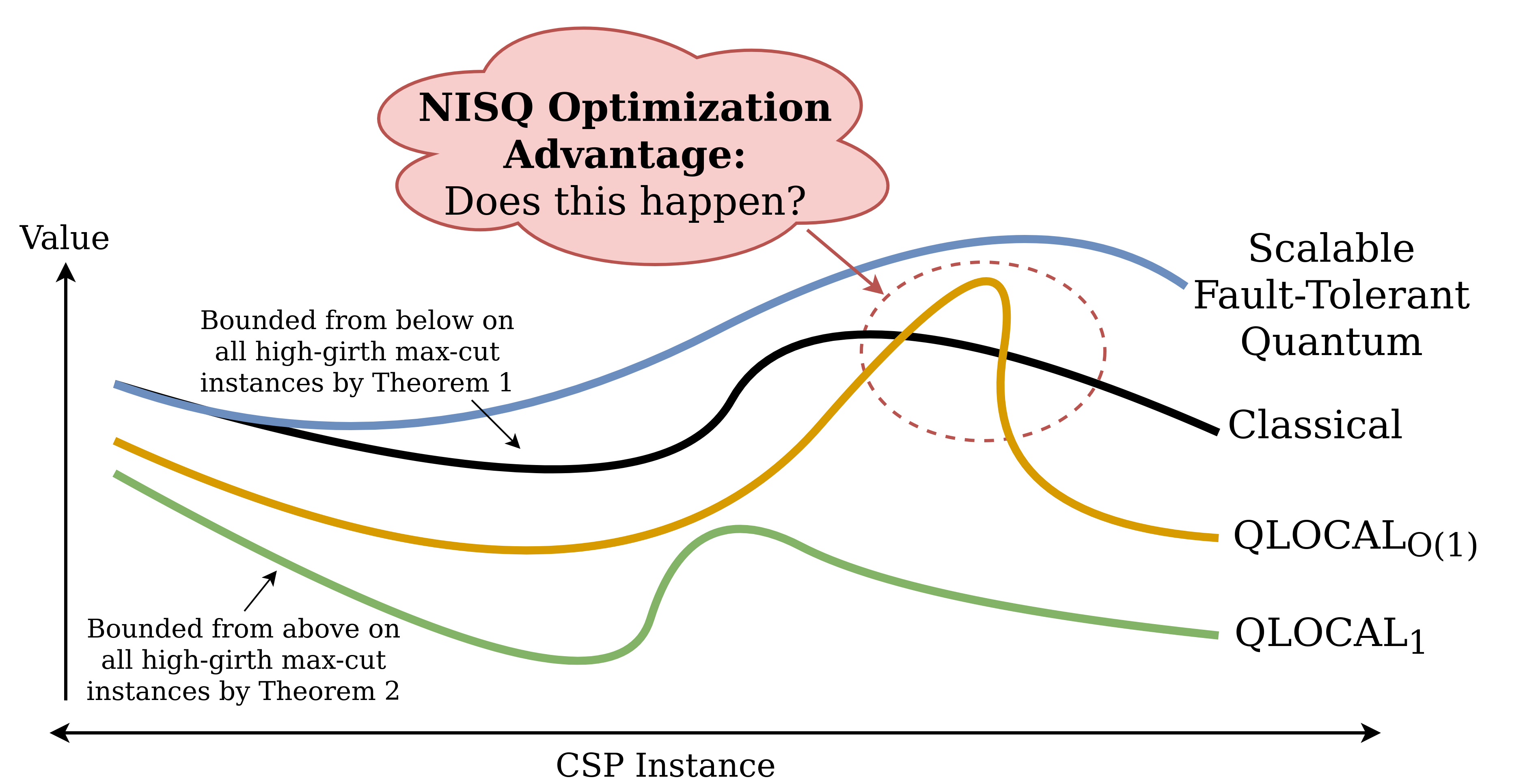
Figure from Barak+ 2021:
Myths about QAOA
| Myth | Explanation |
|---|---|
| MAX-CUT is clearly an interesting problem for quantum advantage | Goemans-Williamson (SDP) is potentially optimal (if Unique Games Conjecture is true). There may be families of graphs where quantum computing can help; but other problems have much bigger gaps between best classical algorithm and limits of approximation. |
| VQE is the same as QAOA | (This section could be improved) VQE is a routine for finding the minimum eigenvalue of a “quantum” Hamiltonian (e.g. electronic structure problem). The variational method is required because we can’t evaluate the Hamiltonian classically. In QAOA, by contrast, the Hamiltonian can be represented classically, but the best solution is not known. Stuart Hadfield refers to this distinction as non-diagonal eigenvalue problem vs diagonal eigenvalue problem. See more information about variational quantum algorithms here. However, one can use QAOA-like algorithms on quantum Hamiltonians; see Anshu+ 2020, Anshu+ 2021. |
| The expected performance is what matters | You really want the highest value the QAOA returns; when you run the experiment many times, you take the best one, not the average one. But we use the average because it’s easier to calculate, and bound the chance of higher performance with tail bounds. (Caveat: at high enough \(n\) and \(p\), there may be concentration – basically every bitstring you sample will achieve exactly the expected performance.) The QAOA may also perform well even if the overlap with optimal value is low. |
| QAOA is just adiabatic computation | Although there are many similarities, there are settings where QAOA improves upon adiabatic computation. See Zhou+ 2018 and also Brady+ 2021. Other comparisons bound the depth \(p\) for QAOA to approximate adiabatic computation, and compare the control strategies (Bapat+ 2018). |
| Using QAOA gives quantum advantage | Although sampling from a \(p=1\) QAOA distribution is not possible classically (Farhi+ 2016), simply using QAOA does not necessarily mean you are calculating things classical computers cannot. In fact, there are no examples (yet?) of provable quantum advantage using QAOA on an optimization problem. In fact, Sreedhar+ 2022 show that classical approximations of the QAOA work equally well as standard QAOA at least for randomly generated MaxCut on Erdos Renyi graph instances and Exact Cover 3 instances. |
| QAOA is a limited model of computation | QAOA, with the right parameters, has been shown to be universal for quantum computation, even on a one-dimensional line of qubits (Lloyd 2018). How it’s done: QAOA can be used to implement “broadcast quantum cellular automaton” dynamics, which is universal for quantum computation. |
Have more to add? Edit this page (button on the left) or email Kunal Marwaha at marwahaha@berkeley.edu.